Machine Learning on Embedded (Part 5)

_Note: This post is the fourth in the series. Here you can find part 1, part 2, part 3 and part 4

Intro

In the previous post part 4, I’ve used x-cube-ai with the STM32F746 to run a tflite model and benchmark the inference performance. In that post I’ve found that the x-cube-ai is ~12.5x faster compared to TensorFlow Lite for microcontrollers (tflite-micro) when running on the same MCU. Generally, the first 4 posts were focused on running the model inference on the edge, which means running the inference on the embedded MCU. This actually is the most important thing nowadays, as being able running inferences on the edge on small MCUs means less consumption and more important that are not rely on the cloud. What is cloud? That means that there is an inference accelerator in cloud, or in layman terms the inference is running on a remote server somewhere on the internet.

One thing to note, is that the only reason I’m using the MNIST model is for benchmarking and consistency with the previous post. There’s no any real reason to use this model in a scenario like this. The important thing here is not the model, but the model’s complexity. So any model with the some kind of complexity that matches your use-case scenario can be used. But as I’ve said since I’ve used this model in the previous posts, I’ll use it also here.

So, what are the benefits of running the inference on the cloud?

Well, that depends. There are many parameters that define a decision like this. I’ll try to list a few of them.

It might be faster to run an inference on the cloud (that depends also on other parameters though).
The MCU that you already have (or you must use) is not capable to run the inference itself using e.g. tflite-micro or another API.
There is a robust network
The time that the cloud inference to be run (including the network transactions) is faster than running on the edge (=on the device)
If the target device runs on battery it may be more energy efficient to use a cloud accelerator
It’s possible to re-train your model and update the cloud without having to update the clients (as long the input and output tensors are not changed).

What are the disadvantages on running the inference on the cloud?

You need a target with a network connection
Networks are not always reliable
The server hardware is not reliable. If the server fails, all the clients will fail
The cloud server is not energy efficient
Maintenance of the cloud

If you ask me, the most important advantage of edge devices is that they don’t rely on any external dependencies. And the most important advantage of the cloud is that it can be updated at any time, even on the fly.

On this post I’ll focus on running the inference on the cloud and use an MCU as a client to that service. Since I like embedded things the cloud tflite server will be a Jetson nano running in the two supported power modes and the client will be an esp8266 NodeMCU running at 160MHz.

All the project file are in this repo:

https://bitbucket.org/dimtass/jetson-nano-tflite-mnist

Now let’s dive into it.

Components

Let’s have a look in the components I’ve used.

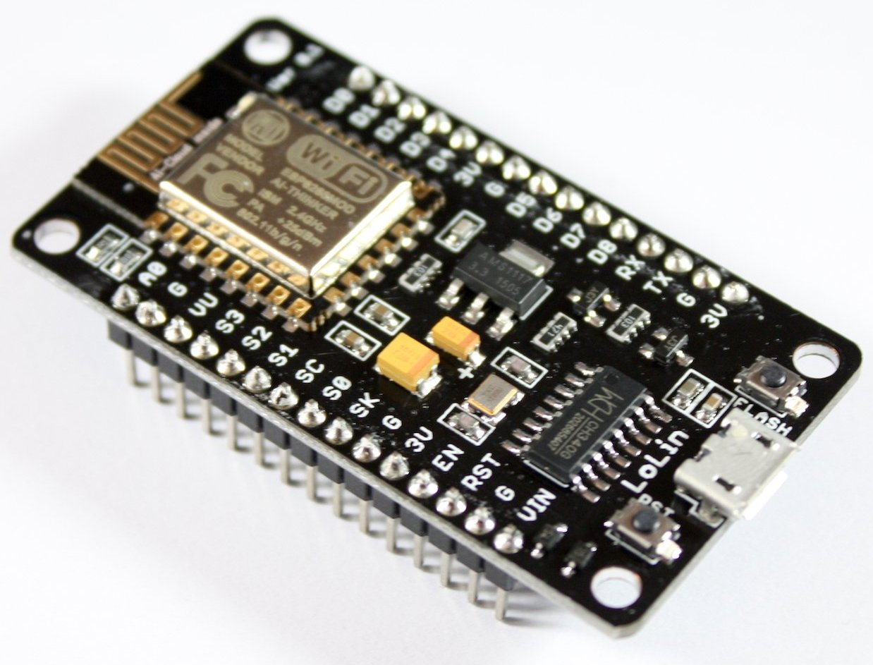
ESP8266 NodeMCU

This is the esp8266 module with 4MB flash and the esp8266 core which can run up to 160MHz. It has two SPI interfaces, one used for the onboard EEPROM and one it’s free to use. Also it has a 12-bit ADC channel which is limited to max 1V input signals. This is a great limitation and we’ll see later why. You can find this on ebay sold for ~1.5 EUR, which is dirt cheap. For this project I’ll use the Arduino library to create a TCP socket that connects to a server, sends an input array and then retrieves the inference result output.

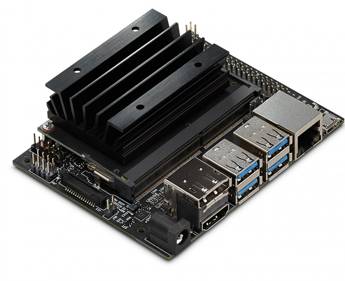
Jetson nano development board

The jetson nano dev board is based on a Quad-core ARM Cortex-A57 running @ 1.4GHz, with 4GB LPDDR4 and an NVIDIA Maxwell GPU with 128 CUDA cores. I’m using this board because the tensorflow-gpu (which contains the tflite) supports its GPU and therefore it provides acceleration when running a model inference. This board doesn’t have WiFi or BT, but it has a mini-pcie connector (key-E) so you’re able to connect a WiFi-BT module. In this project I will just use the ethernet cable connected to a wireless router.

The Jetson nano supports two power modes. The default mode 0 is called MAXN and the mode 1 is called 5W. You can verify on which mode your CPU is running with this command:

nvpmodel -q

And you can set the mode (e.g. mode 1 - 5W) like this:

        
# sets the mode to 5W
sudo nvpmodel -m 1

# sets the mode to MAXN
sudo nvpmodel -m 0

I’ll benchmark both modes in this post.

My workstation

I’ve also used my development workstation in order to do benchmark comparisons with the Jetson nano. The main specs are:

Ryzen 2700x @ 3700MHz (8 cores / 16 threads)
32GB @ 3200MHz
GeForce GT 710 (No CUDA 🙁 )
Ubuntu 18.04
Kernel 4.18.20-041820-generic

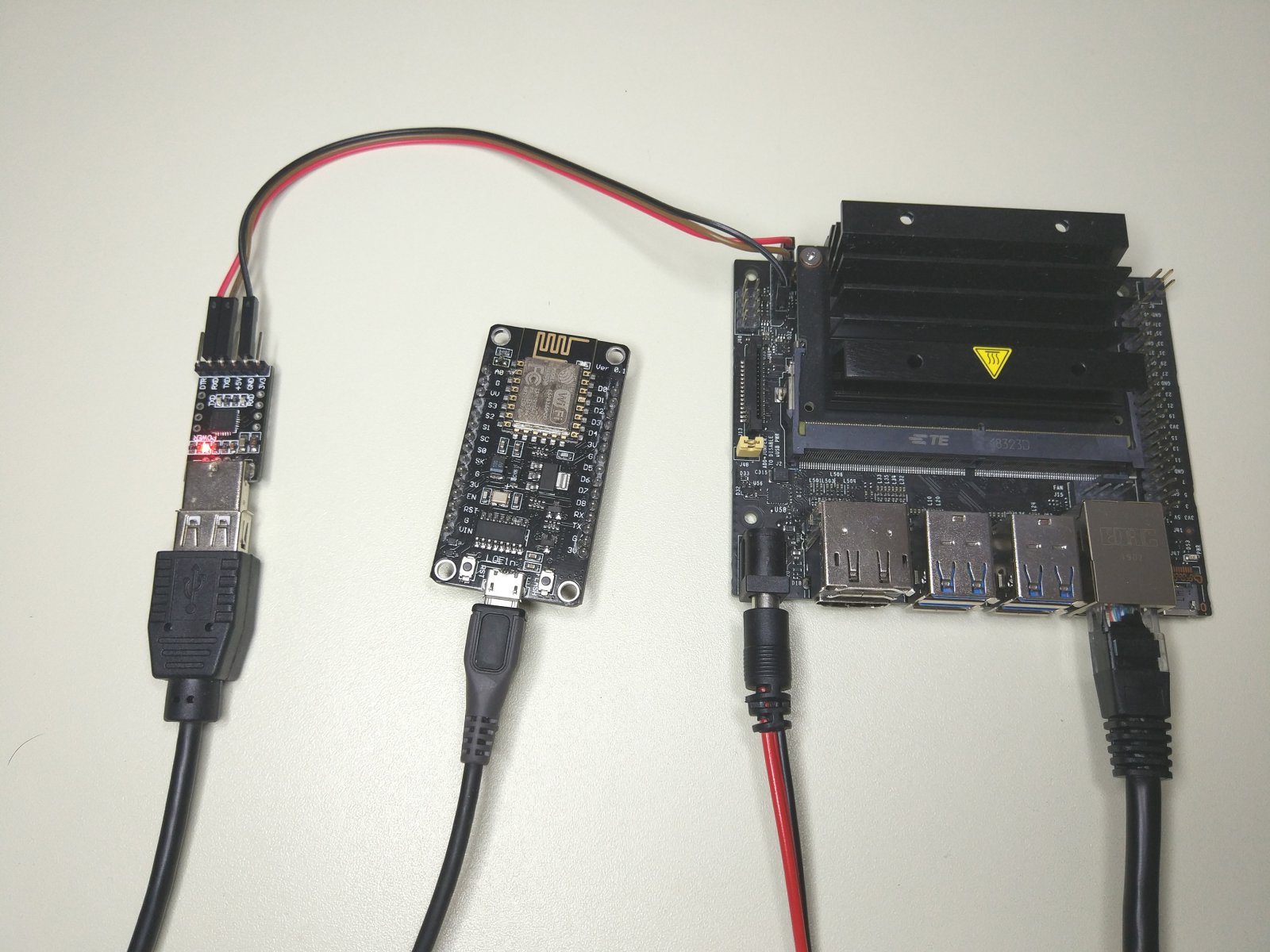
Network setup

This is the network setup I’ve used for the development and testing/benchmarking the project. The esp8266 is connected via WiFi on the router and the workstation (2700x) and the jetson nano are connected via Ethernet ( in the drawing replace TCP = ETH! ).

This is a photo of the development setup.

Repo details

In the repo you’ll find several folders. Here I’ll list what each folder contains. I suggest you also read the README.md file in the repo as it contains information that might not be available here and also the README file will be always updated.

./esp8266-tf-client: This folder contains the firmware for the esp8266
./jupyter_notebook: This folder contains the .ipynb jupyter notebook which you can use on the server and includes the TfliteServer class (which will be explained later) and the tflite model file (mnist.tflite).
./schema: The flatbuffers schema file I’ve used for the communication protocol
./tcp-stress-tool: A C/C++ tool that I’vewritten to stress and benchmark the tflite server.

esp8266 firmware

This folder contains the source code for the esp8266 firmware. To build the esp8266 firmware open the esp8266-tf-client/esp8266-tf-client.ino with Arduino IDE (version > 1.8). Then in the file you need to change a couple of variables according to your network setup. In the source code you’ll find those values:

#define SSID "SSID"
#define SSID_PASSWD "PASSWORD"
#define SERVER_IP "192.168.0.123"
#define SERVER_PORT 32001

You need to edit them according to your wifi network and router setup. So, use your wifi router’s SSID and password. The SERVER_IP is the IP of the computer that will run the python server and the SERVER_PORT is the server’s port and they both need to be the same also in the python script. All the data in the communication between the client and the server are serialized with flatbuffers. This comes with quite a significant performance hit, but it’s quite necessary in this case. The client sends 3180 bytes on every transaction to the server, which are the serialized 784 floats for each 28x28 byte digit. Then the response from the server to the client is 96 bytes. These byte lengths are hardcoded, so if you do any changes you need also to change he definitions in the code. They are hard-coded in order to accelerate the network recv() routines so they don’t wait for timeouts.

By default this project assumes that the esp8266 runs at 160MHz. In case you change this to 80MHz then you need also to change the MS_CONST in the code like this:

#define MS_CONST 80000.0f

Otherwise the ms values will be wrong. I guess there’s an easier and automated way to do this, but yeah…

The firmware supports 3 serial commands that you can send via the terminal. All the commands need to be terminated with a newline. The supported commands are:

Command description

TEST: Sends a single digit inference request to the server and it will print the parsed response
START=<SECS>: Triggers a TCP inference request from the server every <SECS>. Therefore, if you want to poll the server every 5 secs then you need to send this command over the serial to the esp8266 (don’t forget the newline in the end). For example, this will trigger an inference request every 5 seconds: START=5.
STOP: Stops the timer that sends the periodical TCP inference requests

To build and upload the firmware to the esp8266 read the README.md of the repo.

Using the Jupyter notebook

I’ve used the exact same tflite model that I’ve used in part 3 and part 4. The model is located in ./jupyter_notebook/mnist.tflite. You need to clone the repo on the Jetson nano (or your workstation is you prefer). From now on instead of making a distinction between the Jetson nano and the workstation I’ll just refer to them as the cloud as it doesn’t really make any difference. Therefore, just clone the repo to your cloud server. This here is the jupyter notepad on bitbucket.

Benchmarking the inference on the cloud

The important sections in the notepad are 3 and 4. Section 3 is the Benchmark the inference on the Jetson-nano. Here I assume that this runs on the nano, but it’s the same on any server. So, in this section I’m benchmarking the model inference with a random input. I’ve run this benchmark on both my workstation and the Jetson nano and these are the results I got. For reference I’ll also add the numbers with the edge inference on the STM32F7 from the previous post using x-cube-ai.

Cloud server	ms (after 1000 runs)
My workstation	0.206410
Jetson nano (MAXN)	0.987536
Jetson nano (5W)	2.419758
STM32F746 @ 216MHz	76.754
STM32F746 @ 288MHz	57.959

The next table shown the difference in performance between all the different benchmarks.

	STM@216	STM@288	Nano 5W	Nano MAXN	2700x
STM@216	1	1.324	31.719	77.722	371.852
STM@288	0.755	1	23.952	58.69	280.795
Nano 5W	0.031	0.041	1	2.45	11.723
Nano MAXN	0.012	0.017	0.408	1	4.784
2700x	0.002	0.003	0.085	0.209	1

An example how to read the above table is that the STM32F7@288 is 1.324x faster than STM32F7@216. Also Ryzen 2700x is 371.8x times faster. Also the Jetson nano in MAXN mode is 2.45x times faster that the 5W mode, e.t.c.

What you should probably keep from the above table is that Jetson nano is ~32x to 78x times faster than the STM32F7 at the stock clocks. Also the 2700x is only ~4.7x times faster than nano in MAXN mode, which is very good performance for the nano if you think about its consumption, cost and size.

Therefore, the performance/cost and performance/consumption ratio is far better on the Jetson nano compared to 2700x. So it makes perfect sense to use this as a cloud tflite server. One use-case of this scenario is having a cloud accelerator running locally on a place that covers a wide area with WiFi and then having dozens of esp8266 clients that request inferences from the server.

Benchmarking the tflite cloud inference

To run the server you need to run the cell in section 4. Run the TCP server. First you need to insert the correct IP of the cloud server. For example my Jetson nano has the IP 192.168.0.86. Then you run the cell. The other way is you can edit the jupyter_notebook/TfliteServer/TfliteServer.py file and in this code change the IP (or the TCP if you like also)

        
      
if __name__=="__main__":
srv = TfliteServer('../mnist.tflite')
srv.listen('192.168.0.2', 32001)

Then on your terminal run:

python3 TfliteServer.py

This will run the server and you’ll get the following output.

dimtass@jetson-nano:~/rnd/tensorflow-nano/jupyter_notebook/TfliteServer$ python3 TfliteServer.py
TfliteServer initialized
TCP server started at port: 32001

Now send the TEST command on the esp8266 via the serial terminal. When you do this, then the following things will happen:

esp8266 serializes the 28×28 random array to a flatbuffer
esp8266 connects the TCP port of the server
esp8266 sends the flabuffer to the server
Server de-serializes the flatbuffer
Server converts the tensor from (784,) to (1, 28, 28, 1)
Server runs the inference with the input
Server serializes the output it in a flatbuffer (including the time in ms of the inference operation)
Server sends the output back to the esp8266
esp8266 de-serializes the output
esp8266 outputs the result

This is what you get from the esp8266 serial output:

        
      
Request a single inference...
======== Results ========
Inference time in ms: 12.608528
out[0]: 0.080897
out[1]: 0.128900
out[2]: 0.112090
out[3]: 0.129278
out[4]: 0.079890
out[5]: 0.106956
out[6]: 0.074446
out[7]: 0.106730
out[8]: 0.103112
out[9]: 0.077702
Transaction time: 42.387493 ms

In this output the inference time in ms is the time in ms that the cloud server spend to run the inference. Then you get the array of the 10 predictions for the output and finally the Transaction time is the total time of the whole procedure. The total time is the time that steps 1-9 spent. At the same time the output of the server is the following:

        
      
==== Results ====
Hander time in msec: 30.779839
Prediction results: [0.08089687 0.12889975 0.11208985 0.12927799 0.07988966 0.10695633
0.07444601 0.10673008 0.10311186 0.07770159]
Predicted value: 3

The handler time in msec is the time that the TCP reception handler used (see: jupyter_notebook/TfliteServer/TfliteServer.py and the FbTcpHandler class.

From the above benchmark with the esp8266 we need to keep the following two things:

From the 42.38 ms the 12.60 ms was the inference run time, so all the rest things like serialization and network transactions costed 29.78 ms (on the local WiFi network). Therefore, the extra time was 2.3x times more that the inference running time itself.
The total time that the above operation lasted was 42.38 ms and the STM32F7 needed 76.75 ms @ 216MHz (or 57.96 @ 288MHz). That means the the cloud inference is 1.8x and 1.36x times faster.

Finally, as you probably already noticed, the protocol is very simple, so there are no checksums, server-client validation and other fail-safe mechanisms. Of course, that’s on purpose, as you can imagine. Otherwise, the complexity would be higher. But you need to consider those things if you’re going to design a system like this.

Benchmarking the tflite server

The tflite TCP server is just a python TCP socket listener. That means that by design it has much lower performance compared to any TCP server written in C/C++ or Java. Despite the fact that I was aware of this limitation, I’ve chosen to go with this solution in order to integrate the server easily in the jupyter notebook and it was also much faster to implement. Sadly, I’ve seen a great performance hit with this implementation and I would like to investigate a bit further (in the future) and verify if that’s because of the python implementation or something else. The results were pretty bad especially for the Jetson nano.

In order to test the server, I’ve written a small C/C++ stress tool that I’ve used to spawn a user-defined number of TCP client threads and request inferences from the server. Because it’s still early in my testing, I assume that the gpu can only run one inference per time, therefore there’s a thread lock before any thread is able to call the inference function. This lock is in the jupyter_notebook/TfliteServer/TfliteServer.py file in those lines:

        
      
tfliteLock.acquire()
output_data, time_ms = runInference(resp.Input().DigitAsNumpy())
tfliteLock.release()

One thing I would like to mention here is that I’m not lazy to investigate in depth every aspect of each framework, it’s just that I don’t have the time, therefore I do logical assumptions. This is why I assume that I need to put a lock there, in order to prevent several simultaneous calls in the tensorflow API. Maybe this is handled in the API, I don’t know. Anyway, have in mind that’s the reason this lock there, so all the inferences requests will block and wait until the current running inference is finished.

So, the easiest way to run some benchmarks is to use run the TfliteServer on the server. First you need to edit the IP address in the __main__ function. You need to use the IP of the server, or 127.0.0.1 if you run this locally (even when I do this locally I use the real IP address). Then run the server:

cd jupyter_notebook/TfliteServer/
python3 TfliteServer.py

Then you can run the client and pass the server IP, port and number of threads in the command line. For example, I’ve run both the client and server on my workstation, which has the IP 192.168.0.2, so the command I’ve used was:

cd tcp-stress-tool/
./tcp-stress-tool 192.168.0.2 32001 500

This will spawn 500 clients (each on its own thread) and request an inference from the python server. Because the output is quite big, I’ll only post the last line (but I’ve copied some logs in the results/ folder in the repo).

        
      
This tool will spawn a number of TCP clients and will request
the tflite server to run an inference on random data.
Warning: there is no proper input parsing, so you need to be
cautious and read the usage below.

Usage:
tcp-stress-tool [server ip] [server port] [number of clients]

Using:
server ip: 192.168.0.2
server port: 32001
number of clients: 500

Spawning 500 TCP clients...
[thread=2] Connected
[thread=1] Connected
[thread=3] Connected

...

----------------------
Total elapsed time: 31228.558064 ms
Average server inference time: 0.461818 ms

The output means that 500 TCP transactions and inferences were completed in 31.2 secs with average inference time 0.46 ms. That means the total time for the inferences were 23 secs and the rest 8.2 secs were spend in the comms and serializing the data. These 8.2 secs seem a bit too much, though, right? I’m sure that this time should be less. On the Jetson nano it’s even worse, because I wasn’t able to run a test with 500 clients and many connections were rejected. Any number more that 20 threads and python script can’t handle this. I don’t know why. In the results/ folder you’ll find the following test results:

tcp-stress-jetson-nano-10c-5W.txt
tcp-stress-jetson-nano-50c-5W.txt
tcp-stress-jetson-nano-50c-MAXN.txt
tcp-stress-output-workstation-500c.txt

As you can guess from the filename, Xc is the number of threads and for Jetson nano there are results for both modes (MAXN and 5W). This is a table with all the results:

Test	Threads	Total time ms	Avg. inference ms
Nano 5W	10	1057.1	3.645
Nano 5W	20	3094.05	4.888
Nano MAXN	10	236.13	2.41
Nano MAXN	20	3073.33	3.048
2700x	500	31228.55	0.461

From those results, I’m quite sure that there’s something wrong with the python3 TCP server. Maybe at some point I’ll try something different. In any case that concludes my tests, although there’s a question mark as regarding the performance of the Jetson nano when it’s acting as tflite server. For now, it seems that it can’t handle a lot of connections (with this implementation), but I’m quite certain this will be much different if the server is a proper C/C++ implementation.

Conclusions

With this post I’ve finished the main tests around ML I had originally on my mind. I’ve explored how ML can be used with various embedded MCUs and I’ve tested both edge and cloud implementations. At the edge part of ML, I’ve tested a naive implementation and also two higher level APIs (the TensorFlow Lite for Microcontrollers API and also the x-cube-ai from ST). For the cloud part of ML, I’ve tested one of the most common and dirt cheap WiFi enabled MCUs the esp8266.

I’ll mention here once again that, although I’ve used the MNIST example, that doesn’t really matter. It’s the NN model complexity that matters. By that I mean that although it doesn’t make any sense to send a 28x28 tensor from the esp8266 to the cloud for running a prediction on a digit, the model is still just fine for running benchmarks and make conclusions. Also this (784,) input tensor, stresses also the network, which is good for performance tests.

One thing that you might wondering at this point is, which implementation is better? There’s no a single answer for this. This is a per case decision and it depends on several parameters around the specific requirements of the project, like cost, energy efficiency, location, environmental conditioons and several other things. By doing those tests though, I now have a more clear image of the capabilities and the limitations of the current technology and this is a very good thing to have when you have to start with a real project development. I hope that the readers who gone all the posts of this series are able to make some conclusions about those tools and the limitations; and based on this knowledge can start evaluating more focused solutions that fit their project’s specs.

One thing that’s also important, is that the whole ML domain is developing really fast and things are changing very fast, even in next days or even hours. New APIs, new tools, new hardware are showing up. For example, numerous hardware vendors are now releasing products with some kind of NN acceleration (or AI as they prefer to mention it). I’ve read a couple of days ago that even Alibaba released a 16-core RISC-V Processor (XuanTie 910) with AI acceleration. AmLogic released the A311D. Rockchip released the RK3399Pro. Also, Gyrfalcon released the Lightspeeur 2801S Neural Accelerator, to compete Intel’s NCS2 and Google’s TPU. And many more chinese manufactures will release several other RISC-V CPUs with accelerators for NN the next few weeks and months. Therefore, as you can see the ML on the embedded domain is very hot.

I think I will return from time to time to the embedded ML domain in the future to sync with the current progress and maybe write a few more posts on the subject. But the next stupid-project will be something different. There’s still some clean up and editing I want to do in the first 2 posts in the series, though.

I hope you enjoyed this series as much as I did.

Have fun!