Machine Learning on Embedded (Part 1)

Intro

Note: This post is the first in the series. Here you can find part 2, part 3, part 4 and part 5.

Since 2015 I was following the whole machine learning hype closely and after 4 years I can finally say that is mature enough for me to get involved and try to play and experiment with it in the low/mid embedded domain. Although it’s exciting to get immediately involved to new techs, I believe that engineers should just keep an eye on the ones that seem to be valuable in the future or have potential to grow into something that can be used on their domain. But at the same time engineers must be moderate and wait for the hype to fade and then get the real valuable information. This is what happened with machine learning in my case. Now I finally feel that it’s the right time to dig in this domain more seriously and that the tools and frameworks are mature and simple to use.

And this bring us to the fact that, it’s different to implement and develop the tools and it’s a different thing to use them to solve a problem. Until now, many engineers worked hard on the development of these tools and now it’s much easier for us to just use them to solve problems. Keras, for example, it’s exactly that. It’s one really mature and beautiful framework to use and now it’s very stable. On the other hand, when you wait for this to happen, then you have a more steep learn curve in front of you, so from time to time it’s good to be updated with what’s going on in the domains that you’re interested.

Anyway, this time I’ve decided to make a completely stupid project to find the limits and the use cases of ML in the embedded world. Well, don’t get me wrong that’s not a research, it’s just evaluating the current status of the tools and how they perform with the current low embedded technologies. Nowadays, when most engineers hear embedded they think of some kind ARM application CPU that runs Linux on a SBC. Well, sure, that’s embedded too and there are many of those SBCs these days and they are really cheap, but embedded is also those dirt cheap 8, 16, 32-bit RISC MCUs and also the Cortex-M series.

Let’s make some assumptions for the rest of this post. Let’s assume that low embedded is everything that is equal or less than a Cortex-M MCUs and high embedded all the rest application CPUs that can actually run Linux. I know that there also some smaller MMU-less MCUs that can run Linux, but let’s forget about that now. Also from now on I’ll refer to machine and deep learning as ML, just for convenience. Although the terminology on the field is getting standardized I’ll try to keep it simple, even if I’m not using the proper convention in some cases. Otherwise this post will become like those that I was reading my self in the beginning that were really hard to follow. So, although there are some differences, let’s keep it simple. AI, deep learning, machine learning… I’ll just use ML! Also I’ll refer to a single neural as a neural or a node. Finally, I’ll refer to neural network as NN.

This article will be split in 4 or 5 different posts. The first one (this one) will have some very generic information about ML and NN; but not in depth, as this is not the purpose of this post series. Also in this post we’ll implement a very simple NN with a single node with 3 inputs and 1 output and then run some benchmarks in various MCUs and analyze the results.

In the second part I’ll use the same MCUs but with a bit more complex NN that has the same inputs, but a hidden layer with 32 nodes and 1 output. This NN will be more accurate in its predictions (as we’ll see), compared to the simple NN; but at the same time it will need more processing time to run the forward prediction. Please don’t expect to learn the terminology and details on ML here, but it will be much easier to follow if you already know some basic things around NN.

Excited already? No? Well, don’t forget it’s a stupid project. There’s always a small excitement in doing something useless. So, let’s move on.

Components

Spoiler. For me, one of the most interesting thing in this stupid project was the amount of the different boards that I’ve used to run those benchmarks. I think what I liked most was the fact that I was able to test all these different boards with the same code. For sure, the stm32f103 (blue-pill) was more optimized as I’ve used my own low level cmake template, but nevertheless I enjoyed having most of my boards running the same neural network code. Well, I didn’t used any of my PSoC 4 & 5, STM8, LPC1110, LPC1768 and a few other boards I have around, but I didn’t have more time to spend on this. Maybe at some later point I’ll add the benchmark for those, too.

STM32F103C8T6 (aka blue-pill)

This is my favorite board and my reference, so it couldn’t miss the party. I’ve run the benchmarks @72MHz and then I’ve overclocked the MCU @128MHz.

STM32F746G

This is actually the STM32 F7 discovery board here, which is a cute development board with a lot of peripherals and cool stuff on it, but in this case I’ve only use a serial port and a gpio pin. As I like to overclock the stm32s, I’ve managed to overclock this mcu @295MHz. After that it didn’t work for me.

Arduino Uno

I guess I don’t need to write more about this. Everybody knows it. It runs on a ATmega328p and it’s the slowest MCU in this comparison.

Arduino Leonardo

This is another Arduino variant with the ATmega32 cpu, which is a bit faster than the ATmega328p.

Arduino DUE

This is an arduino board that runs on an Atmel SAM3X8E MCU, which is actually an ARM Cortex-M3 running at 84MHz. Quite fast MCU for its release date back then.

Teensy 3.2

The teensy is a very interesting board. It’s a bit expensive, sure. But it’s almost fully compatible with the Arduino IDE libraries and that makes it ideal for fast prototyping and testing. It’s based on a Cortex-M4 CPU and for the test I’ve used it overclocked @120MHz.

Teensy 3.5

This teensy board is using a Cortex-M4 CPU, too; but it runs on faster clocks. I’ve also used it overclocked @168MHz. The overclocking options for both teensy boards, are coming easy and for free from within the Teensy plugin in the Arduino IDE. I had some issues with one library but nothing difficult to solve. More details in the README.md file on each MCU code folder.

ESP8266-12E

Yep, we all now this board. An L106 32-bit RISC CPU running up to 160MHz.

A simple NN

OK, so let’s now jump to the interesting stuff. Everything that is related to this project and for all the posts are in this github repo:

https://github.com/dimtass/machine-learning-for-embedded

Although it’s not the best thing to have all these different things in one repo, it makes more sense as it makes it easier to maintain and update. During this post series I’ll use different parts from this repo, so everything you see there are not only for the this first post.

Before we begin, in case that you want to learn some basics for NN then you can watch these videos in YouTube (1, 2, 3, 4) and also this playlist.

First let’s start with a simple NN. For this post, we’re going to use a single neural with 3 inputs and 1 output. You can see that in the following picture.

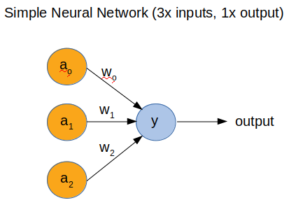
In the above image we see the topology of a simple NN. That has 3x inputs and 1x output. I won’t get into the details of the math. In this case the output is simple to calculate and it’s:

y = a0*w0 + a1*w1 + a2*w2

This is the dot product of a(n) and w(n), where n=1,2,3. Just be aware that a(n) is not a function, it just means a0, a1, a2. The same for w(n). So, a(n) are the inputs and w(n) are the so called weights. You can think that weights are just numbers that their size control the effect that each a(n) has in the output result. The higher the w(n) is the more a(n) affects y.

The output is not y, thought. The output is the sigmoid of y, so:

output = sigmoid(y)

What sigmoid does is that it limits the output between 0 and 1. So the more negative y is then it’s near 0 and the more positive it’s near 1. In the ML world this function is called activation function.

For this project we assume that a(n) is a single binary digit (0 or 1). Therefore, since we have 3 inputs then all the possible combinations are in the following table:

a0	a1	a2
0	0	0
0	0	1
0	1	0
0	1	1
1	0	0
1	0	1
1	1	0
1	1	1

For simplicity, you can think of those inputs as 3 buttons connected to 3 gpio pins on the MCU and their state is either pressedor not pressed. Then depending their state, the output is also a binary value (0 or 1).

Training the model

Training the model means getting a set of inputs that we already know that they produce a specific output and then train the NN according to these. Then we hope/expect that the NN is able to predict the output for unknown inputs that hasn’t been trained on. The training is not done on the target, but it’s done separately on a workstation (or cloud) that has more processing power; and finally only execute the prediction function on the MCU. Although this model is very simple, someone may argue that 2 inputs - 1 output is simpler :p . Although it’s simple enough, we’ll do the training on a workstation as it’s important to use some tools that make the workflow easier.

To do that, is better to use a jupyter notebook to do all the design, training, testing and evaluation. Also Jupyter notebooks are the standard documents that you’ll find in most new github projects. The most simple way to install Jupyter and the other tools we need is using miniconda. I’ll be really quick on this. I’m using Ubuntu, so the following commands are for that OS.

Download miniconda from here
Install miniconda

Create a new environment and install the tools you’ll need

  
  # Create a new environment
  conda create -n nn-env python
  # Activate the environment
  conda activate nn-env
  # Now install those packages to that environment
  conda install -c conda-forge numpy
  conda install -c conda-forge jupyter
  conda install -c conda-forge scikit-learn
  conda install -c conda-forge tensorflow-gpu
  conda install -c conda-forge keras

Not all of the above packages needed for this example, but we’ll use them later.

Next git clone the repo for this project and run Jupyter.

git clone git@github.com:dimtass/machine-learning-for-embedded.git
cd machine-learning-for-embedded
jupyter notebook &

If everything goes right, then now you should be able to see the web-interface from Jupyter in your browser. If not, then I guess you need to do some google-fu. In this web interface you would see a folder with the name jupyter_notebooks. Just double click on that and there you’ll find all the notebooks for this project. The one we need for this post is the Simple python NN.ipynb. Just click on that.

What you see in there is some mix of markdown text and python code. For the simple cases of the first two parts we’re going to implement the NN with just python code, without using any advanced library like tensorflow or keras. The reason for this is that we can write code that we can later convert to simple C and run tests on the different MCUs.

Again, I won’t go into the details of Jupyter notebooks and python. I guess there are plenty of tutorials in internet that are much better from any explanation I can provide.

Let’s see the notepad now.

Note: In case you just want to view the notebook and evaluate your results, you don’t have to install Jupyter, but instead you can just view the notebook in the github repo here.

First we import some functions from numpy to simplify the code. Then we create a NeuralNetwork class that is able to train and evaluate our simple NN. Then we create a training set for our binary inputs. As we’ve seen before, 3 binary inputs have 8 possible combinations and we choose to use a train set of 4 inputs. That means that we’ll train our NN with only 4 out of 8 combinations and then expect the NN to be able to predict the rest by itself. So we train with the 50% of the possible values.

Then we create an array with the 4 inputs and the 4 outputs. After that we initialize the NeuralNetwork class and view the random weights. A note here is that the weights always have random values in the beginning. The meaning of training is to calculate those weights (if you prefer the mathematical approach is to find where the slope of the function, I’ve mentioned before, is minimum or ideally zero). Another note is that when you run this notebook in your browser you may get different values after each training (you shouldn’t but you may). Those values should be similar to the ones in the notebook, but they also might differ a bit. In this case, if you just want to evaluate your results with the C code that runs on the MCUs then have in mind that you may need to change the weights in the MCU code according to your weights. By default, the weights in the C code are the ones that you get in the repo’s notebooks without execute any cells.

Finally, we train the model to calculate the weights and then we evaluate the model with all the possible input combinations. For convenience I’m copying my results here:

  
[0 0 0] = [0.5]
[0 0 1] = [0.009664]
[0 1 0] = [0.44822538]
[0 1 1] = [0.00786466]
[1 0 0] = [0.99993704]
[1 0 1] = [0.99358931]
[1 1 0] = [0.9999225]
[1 1 1] = [0.99211997]

From the above output we see that for the values that we used during training the predictions are very accurate. This output is from the stm32f203, as you’ll find out all the Arduino compiled code don’t have that floating point precision when you convert the doubles to strings. As I’ve mentioned before in the output we get values from 0 to 1. That’s the prediction of the NN and the closer is to 0 or 1 then the higher is the possibility that the output has that value (because in this example it happens that we have binary output so it’s 0 or 1 anyways). So in case of the training inputs [[0, 0, 1], [1, 1, 1], [1, 0, 1], [0, 1, 1]] we see that the accuracy is much better compared to the unknown inputs like [0 0 0] and [0 1 0]. Especially the first input it’s not actually possible to say if it’s 0 or 1 as it stands right in the middle. Ouch!

Evaluate on the MCUs

Now that we designed, trained and evaluated our model on the Jupyter notepad we’re going to test the NN on different MCUs.

What is important here is not actually if the prediction really works on the MCUs. I mean that’s just code, of course it will work the same way and you’ll get similar results. You results might differ a bit because as we use doubles that may differ from one architecture to other. What is important though, is the performance !

That’s all about we care eventually, right? And that was the main drive for me to create this project. To find out how do those MCUs perform in simple or more complex NNs? Is it possible to run a NN in real-time? Does it even have a meaning to do that on an MCU? What you should expect? Is it worth it? Can those tiny MCUs give a good performance? What are the limits? Is it maybe better to convert a NN problem to algorithmic in order to run it on a MCU? Are nested ifs, lookup tables, Karnaugh maps still a better alternative? And a lot of other questions.

Just be sure that I’m not going to answer all those things here though, as there are a lot of different parameters per project and use case. But by doing this yourself, you should definitely get an idea of the performance, the potentials and the limits that exist with the current technologies.

The evaluation on the MCUs is split in 3 different cases. We have the stm32f103 that has it’s own code folder in the code-stm32f013 folder. Also the stm32f746 has it’s own code folder (code-stm32f746), as esp8266 and arduino due. For the other arduinos and teensy boards you can use the code-arduinofolder.

Just a parenthesis here. Probably people that read my blog more often, they know that I’m more a baremetal embedded guy. I enjoy doing stuff with more stripped down libraries even CMSIS for the Cortex-M. Although I’m mentioning from time to time that I don’t like using Arduino IDE or HAL libraries, I’ve also mentioned that I find these very useful for cases like this. Prototyping! Therefore, using those tools for prototyping is an excellent choice and a no-brain decision. We need to choose and use our tools wisely and where they fit best every time. So evaluating a case or project on different HW it always make sense to use those tools for prototyping and then write the proper low embedded code where is needed. OK, enough with this parenthesis.

You’ll find details on how to build and run each code on each MCU in the README files in the project folders. Hence, I’ll only mention the serial protocol that I’m using and also how it works in the background.

C code

The c code is really simple for this example. The dot product and the sigmoid function are implemented in the neural_network.h/c files and from the main.c file we just call the prediction() functions (which is just the sigmoid dot() function). The same .h and .c files are used for all the different codes. Also the weights for this example is the double weights[] array in main.c and the inputs are the double inputs[8][3] array again in the main.c function. For now just ignore the double weights_1[32][3] and double weights_2[] arrays, which are used for part 2.

Finally, also two important functions for this example are the benchmark_neural_network() and test_neural_network(). Both are triggered with commands from the serial port. The test function will just print the prediction for all the input combinations in order to compare them with the jupyter notebook and the benchmark function will run a single prediction and at the same time toggle a pin in order to measure the time the function has taken with an oscilloscope.

Supported serial commands

In order to simplify testing I’ve created a couple of commands. In case of stm32 you can connect to the serial port at 115kbps and for the rest MCUs that use the .ino project you need to connect at 9600 bps (anyway it’s either 9600 or 115200).

The supported commands are the following (all commands expect a newline in the end):

TEST=<mode>

where <mode>: 1 or 2

This command will evaluate all the 8 possible inputs by running the prediction using the calculated weights and will print the output. Then you can compare the output with the output from the jupyter notebook.

Mode 1, is using the simple1 NN and its weights. The simple1 NN is the one we use on this post with 3 inputs and 1 output.

Mode 2, is using the simple2 NN and its weights. The simple2 NN is the one that we use on part 2 with 2 inputs, a hidden layer with 32 nodes and 1 output.

Note: If you run the TEST commands on any arduino build firmware you’ll get a bit disappointed as you for some reason the Serial.print function can only print double values with a 2 decimals. That’s a bit crap. I’ve read that there are some ways to fix this, but that it doesn’t really matter. It only matters that the predictions are correct enough. With stm32 that’s not an issue you will get pretty much the same accuracy with the python output.

START=<mode>

where <mode>: 1 or 2 (has the same meaning as before)

This command starts a timer that every 3 seconds will run the prediction function and also toggles a gpio in order to help us to make precision measurements. By default, the prediction is using the first input set [0 0 0]. That doesn’t really matter as it doesn’t affect the computation timing, but you can change it in the code if you like. You can verify that mode 1 is much faster than mode 2, but we’ll have a look at it at the next post.

STOP

The STOP commands just stops the timer that was triggered with the START=<mode> command.

Benchmarks

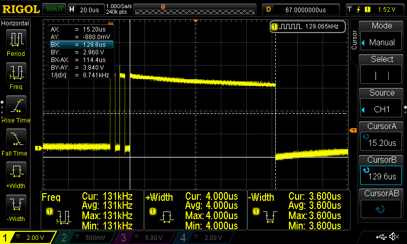
First I need to mention that the best way to measure the time that a code needs to run is by using an oscilloscope and a gpio pin. You can set the pin high just before you run your function, then run the function and then set the pin to low. Then by using the oscilloscope you can calculate the exact time the operation lasted.

There’s a catch though! When toggling a pin, that also takes some time and that time is different for different hardware and even gpio libraries for the same hardware. For that reason in the code you’ll find out that every time I’m toggling the pin twice before run the NN prediction function. That way you can measure the time that those two toggles spend and then subtract the average from the time that the prediction operation lasted. So, you measure the time of the two toggles and if that time is Tt then you measure the time between the HIGH and LOW of the prediction function and the total time spend for the predictions will be:

Tp = Thl - (Tt/2)

where:

Tp: Prediction time
Thl: Time of High-Low transition that includes the prediction function
Tt: Time of the two toggles

Anyway, let’s not complicate things more. The above just helps only when the prediction function time is fast or different MCUs have similar time and you want to remove the overhead of any GPIO handling that may differ between different MCUs.

Note: I’ve included all the oscilloscope screenshots in the screenshots folder in the repo. Therefore, you can have a look on the oscilloscope output for each different MCU as I’m not going to post them all here (there are just too many).

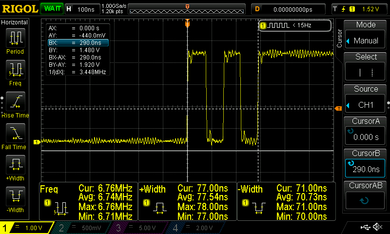
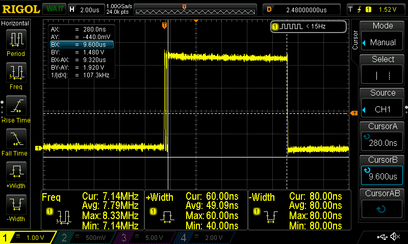
Before posting the table of the results, these are the screenshots for the stm32f103 and the Arduino Uno. The name coding in the screenshots folder is <mcu>-<NN topology>-<frequency>-<capture>.png. That means that for the teensy 3. 2 the ss for that simple example (simple1) and the pin toggle will be teensy_3.2-simple1-120MHz-predict.png. In the next post (part 2) the NN topology will be called simple2.

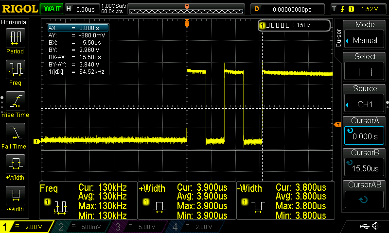
These are the captures for the toggle and prediction for stm32f103 and arduino uno.

stm32f103 @ 128MHz pin toggle time = 290 nsec

stm32f103 @ 128MHz prediction time = 9.38 μsec

Arduino Uno @ 8MHz pin toggle time = 15.5 μsec

Arduino Uno @ 8MHz prediction time = 114.4 μsec

Although you already get a rough idea, the next table summarizes everything.

MCU Pin	toggle time (μsec)	Prediction time (μsec)
stm32f103 @ 72MHz	0.512	16.9
stm32f103 @ 128MHz	0.290	9.38
Arduino Uno @ 8MHz	15.5	114.4
Ard. Leonardo @ 16MHz	21	116
Arduino DUE @ 84MHz	8.8	18.9
ESP8266-12E @ 160MHz	1.58	15.64
Teensy 3.2 @ 120MHz	0.830	11.76
Teensy 3.5 @ 168MHz	0.572	8.84
stm32f746 @ 216MHz	0.157	4.86
stm32f746 @ 295MHz	0.115	3.58

As you can see from the above table the higher the frequency the better the performance (o, really?). I haven’t substracted the pin toggle time from the prediction time! Also note that although the Teensy 3.5 has a better performance from the stm32f103@128MHz the pin toggle time is almost the double… That’s because those arduino libraries are implemented on top of bloated functions, even for just enable/disable a pin. Of course, the overclocked stm32f746 @ 295MHz is by far the fastest in all terms.

Also I’ve noticed something irrelevant with the NN. If you see the ratio of the (Prediction time)/(Pin toggle time), then you get some interesting numbers. Let’s see the following table:

MCU	(prediction time)/(pin toggle time)
stm32f103 @ 72MHz	33
stm32f103 @ 128MHz	32.34
Arduino Uno @ 8MHz	7.38
Ard. Leonardo @ 16MHz	5.52
Arduino DUE @ 84MHz	2.14
ESP8266-12E @ 160MHz	9.89
Teensy 3.2 @ 120MHz	14.16
Teensy 3.5 @ 168MHz	15.45
stm32f746 @ 295MHz	31.13

The above table shows what you can expect from your hardware and how those bloatware arduino libs hurt the overall performance. To be fair though, the NN code is not affected from the libraries, as it’s plain C code. But normally your MCU will also do other tasks and not only run the NN; therefore, everything else that the cpu does affects the NN performance, especially if the code uses bloated libraries. In this case we just toggle a pin and running a timer in the background, nothing else. Well, not true, the stm32f103 actually runs also a few other stuff in the background, but nevertheless it has the best prediction/toggle ratio. The Arduino DUE has the most weird behavior, which doesn’t make sense, but it was consistent. I didn’t even bother to debug that, though. Anyway, the above table is the reason that sometimes I mention that prototyping is completely different from development. Prototyping is proof of concept, and after that going into the low level will bring you the performance. If you don’t care about performance, then sure pick the tool that suits your needs.

Conclusions

From this example we’ve seen that we can actually design, train, evaluate and test a NN with Jupyter and python and then run the forward prediction function on a small MCU. Isn’t that great? Yeah, I know… Using so much resources on those small MCUs to run a 3-input, 1-output NN deserves the title of the stupid project! Anyway, from the last tables we have some interesting results that you can also interpret as you think.

The most interesting is that we can actually use this NN for real-time applications! OK, don’t laugh. I know that this example it’s useless, but you can! Even the 114.4 usec of the Arduino is ok’ish for fast real-time applications. Of course, it depends on the case and the specs. I mean if you expect you inputs to change faster than that, of course you can’t use it. But think buttons for now! 😛

It’s really fast and even Arduino uno can handle this NN, 100 μsec is really fast. Oh, wait. That bring us on another question. If they are buttons then why not created a nested-if function and handle that much much faster.

Even better, why not create lookup table? Maybe even create a Karnaugh map of the inputs/outputs and reduce that to a couple of logic operations. That would work really really fast!

Well, as I said, this is a very simplified example. I mean, this is just for testing and is not meant to do anything really usable. But on the other hand think that what if instead of 3 inputs we had 128? Or 512? Then it would be really difficult to make a Karnaugh map and simplify it. Or we would need to write a ton of if-else cases. But what would happened if we needed to change something in the input or output sets? Then it would be also quite some work in the code. Maybe the lookup table is still a valid and good solution, though. It will cost RAM or FLASH space, but also the weights of the NN will get a lot of space. So you would need to compare how much space each solution would use and then if the NN needs less space then decide if less space is more important than speed execution.

It’s important to realise that ML doesn’t make better every problem we have, neither it’s a magic tool that solves all our engineering problems. It’s a tool that seems to have the potential to solve some issues that it was very complicated to solve before. And it may apply also to problems that we already have solutions for them, but ML may provide some flexibility we didn’t have before.

In the next post here will do the same for a bit more complex NN with 3-inputs, a hidden layer with 32 nodes and 1-output.

Have fun!